

The DevRev platform serves customers across the globe providing an array of features such as ticket deduplication, similarity search, deflection, and retrieval augmented generation. These are built on the foundation of a fast and efficient search system that relies on a scalable multi-tenant vector database. The DevRev platform accommodates freemium users and adopts a usage-based charging model, underscoring the significance of minimizing costs for inactive users. We discussed semantic search and our reasoning for building a vector database in an earlier post here
In this post, we will dive into the choice of algorithm for the DevRev Vector Database. We named our database Honeycomb.
A quick refresher of the problem statement we are trying to solve.
We need an accurate, fast and cost efficient mechanism to assess the similarity of objects based on capturing the meaning.
to accomplish this, the object(text) is mapped to numeric vectors using an embedding model such that objects with similar meaning are placed closer together.
Below is an illustration depicting sentences mapped to vectors in two dimensional space. The query sentence is depicted by a vector shown in green while the other sentences are depicted as vectors shown in blue.
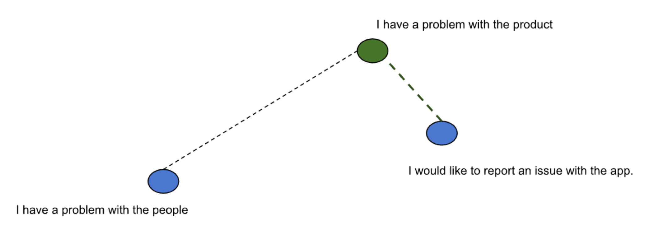
To find sentences similar to the query “I have a problem with the product”, the vector nearest to the vector in green is calculated. k is used to denote the number of matches we want to derive from the search. We have reduced the original search problem to one of finding k vectors nearest to the provided query vector. So we need an algorithm for nearest neighbor search. The algorithm needs to be evaluated against search quality, speed and memory consumption.
Algorithms Considered
Exact K Nearest Neighbor Search
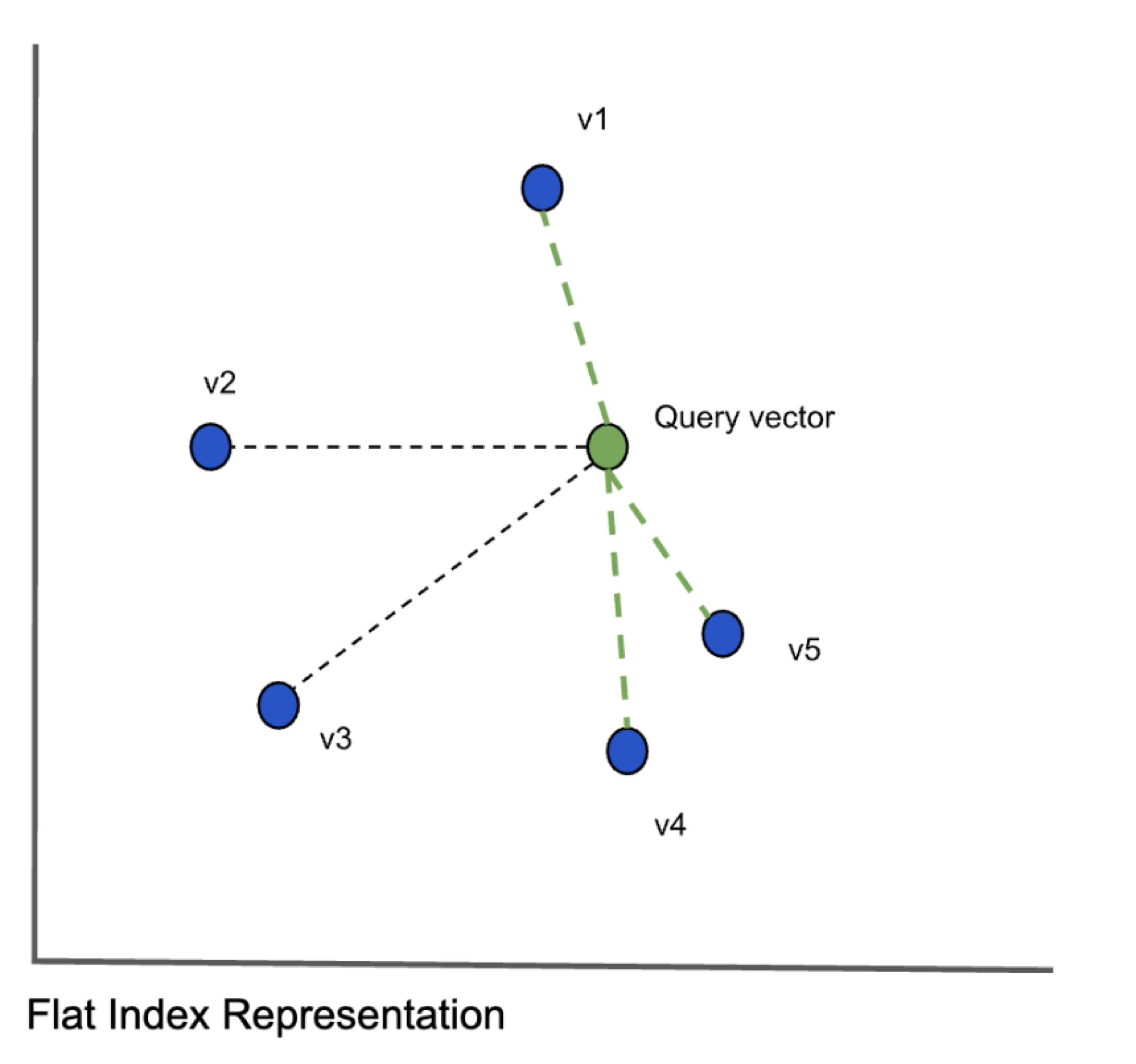
To find the k vectors closest to the query vector, we compare the query vector with every other vector (shown in blue above) and calculate the distances between them. This algorithm is called exact k-nearest neighbors (kNN) search and provides great search quality but the search times could be very large when the number of objects increse. When we scale the data to millions of vectors with hundreds of dimensions, this approach clearly will not scale. It does however provide the highest accuracy. Given the problem with scaling, we have to consider approximate nearest neighbor algorithms which will have reduced accuracy but will significantly speed up the search. There are three main classes of algorithms: hash based, tree based and graph based algorithms.
Locality Sensitive Hashing
The algorithm works by grouping vectors into buckets to maximize hashing collisions. This is contrary to the conventional hash functions which minimize collisions. The intuition is to group all similar items by mapping them to the same key. This algorithm performs badly in terms of both memory consumption as well as speed for vectors with higher dimensionality. The algorithm does poorly even with vectors with 128 dimensions. For our use cases, we definitely need higher dimensionality. So this algorithm will not cut it.
Hierarchical Navigable Small World (HNSW)
HNSW is a proximity graph algorithm The nodes in the graph are connected to other nodes based on their proximity. Euclidean distance is used to measure proximity. The details are described in the paper here
The best way to think of the HNSW algorithm is as a combination of probability skip lists and navigable small world graphs. The skip lists reduce the search space when dealing with large volumes of data. The Navigable small world graph has short and long range links making them very navigable. The small world refers to the fact that the graph can be very large, but the number of hops between any two vertices on the graph is small. The intuition behind this can be understood from the Six degrees of separation idea that states all people are six or fewer social connections away from each other.
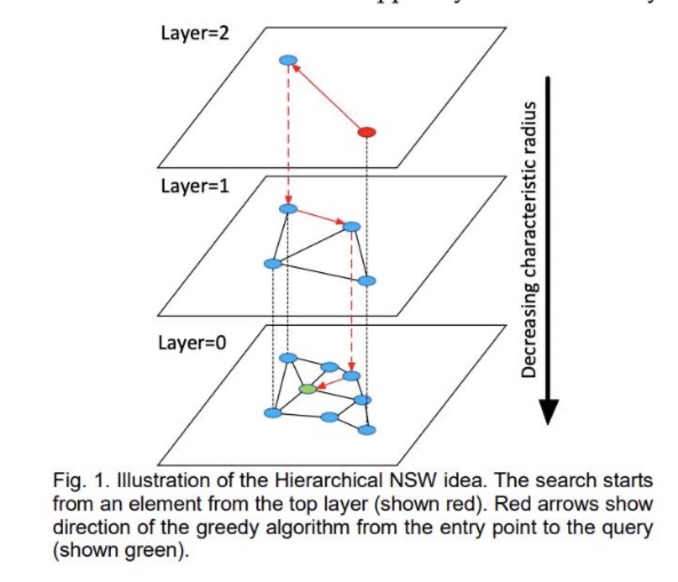 HNSW Algorithm: Copyright:https://arxiv.org/pdf/1603.09320.pdf
HNSW graphs are built by breaking apart the NSW graphs across multiple layers. Each layer eliminates intermediate connections between vertices. The search starts from the highest layer and proceeds to one level below when the local nearest neighbor is greedily found among the layer nodes. The nearest neighbor on the lowest layer is the answer to the query.
There are three key parameters which can be used to adjust the search quality and speed.
- maxConnections: The number of nearest neighbors that each vertex will connect to.
- efSearch: The number of entry points explored between layers during the search.
- efConstruction: The number of entry points explored when building the index.
Increasing these values increases the search quality but it also increases the search time.
The HNSW algorithm can give us great search quality and speed, but the memory consumption is very high. Assuming we set the maxConnections to 64, the algorithm consumes upwards of 2 GB of memory if the model uses a vector with 384 dimensions and the dataset contains 1 million vectors. Given the models we use have higher dimensions and the volume of data we expect to handle is more than 1 million, this will impose very large memory requirements and consequently increased costs when used at scale.
Inverted file Index
The inverted file index is built by clustering vectors to reduce the search space. The vectors are divided into a number of clusters partitioning the search space. The partitioned search space is best depicted using a Voronoi Diagram Each of the vectors falls in one of the cluster partitions and is represented by the centroid value. The query vector is mapped to one of the clusters by calculating the distance between the query vector and centroids of the clusters. The search is then restricted only to the cluster whose centroid is nearest to the query vector.
The Voronoi Diagram below depicts the centroids of the clusters.
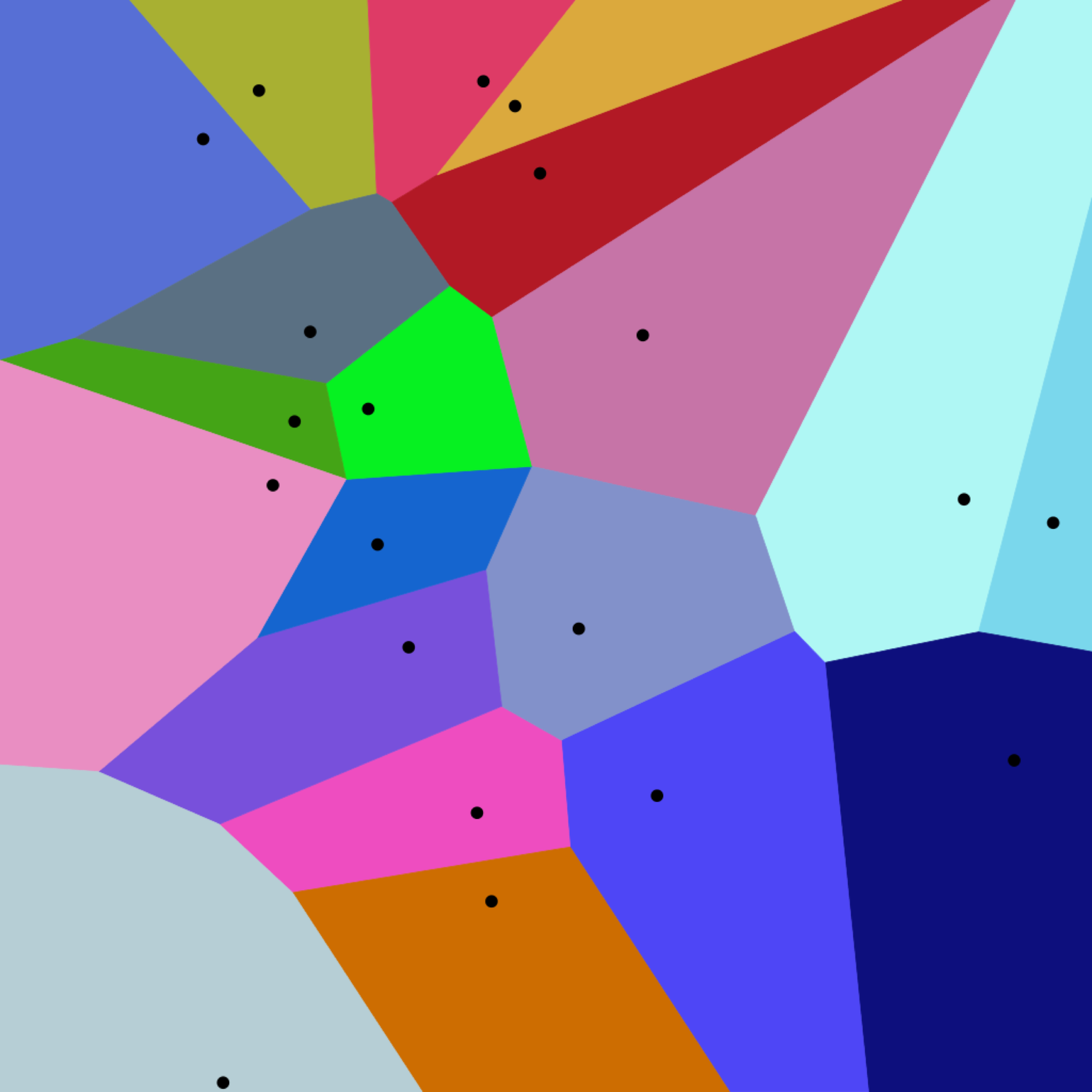 Voronoii Diagram with Euclidean distance
When the query vector happens to fall on the edge separating two clusters, the algorithm may incorrectly map it to the wrong centroid. This is referred to as the edge problem. Increasing the number of nearest clusters we include in the search space mitigates the edge problem.
There are two key parameters we can use to control search quality and speed.
- n_list - The number of clusters to create
- n_probe - The number of clusters to search
Increasing n_list will increase the number of comparisons between the query vector and the centroids, but once a centroid is picked, there are fewer vectors within that cluster. So increasing n_list will increase the search speed.
Increasing n_probe on the other hand will improve search quality by increasing the search scope to include more clusters.
The algorithm has good search quality and speed and also does not consume as much memory.
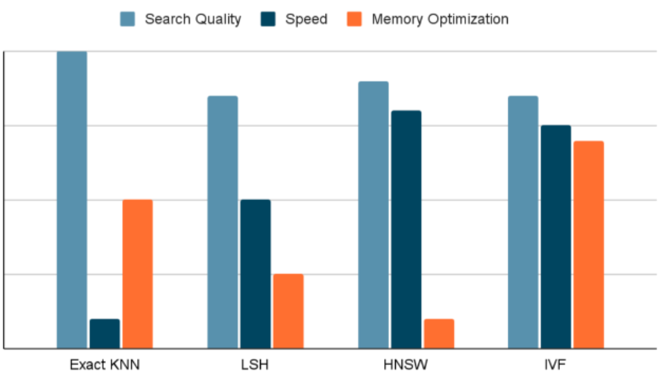
The graph below is a visual summary of our discussion. Given the need to optimize for latency, speed as well as memory usage, an Inverted File Index based algorithm was the best choice to build our vector database
Honeycomb Algorithm
Honeycomb uses a hierarchical IVF index. The index is built by clustering the vectors. The size of every cluster is limited to 1 MB in each layer. The idea behind this is to optimize for search speed. A layered or hierarchical approach is used to narrow the search space. The base layer or layer 0 consists of clustered vectors. The next layer or layer 1 forms clusters based on the centroids of the clusters in layer 0. The cluster size limitation of 1 MB also applies to the next layer. This process of clustering centroids in subsequent layers can continue until we have exactly one cluster. Each cluster is represented by its centroid.
Hierarchical IVF Index
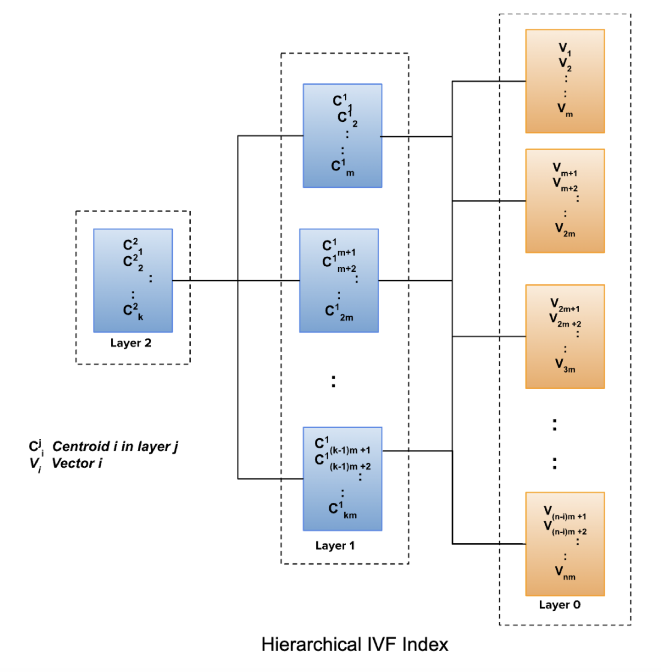
k-means clustering is used to generate the clusters with the number of clusters derived by capping the cluster size to 1MB. The clustering algorithm starts with choosing random centroids and mapping vectors to each of these centroids to form the clusters.
The formula below derives the maximum number of vectors per cluster based on the dimesion.

vector_dimension - The dimension of the vector chosen based on the embedding model. Every vector is represented as float32
The limits on cluster size facilitate the use of a cache for the root layer with centroids to speed up computations. An inexpensive storage is chosen for the base layer containing the vectors. Honeycomb employs a combination of exact kNN and the hierarchical clustering to balance search quality, speed and memory consumption.